Repository navigation
Expand file tree
/
Copy path1_1_matplotlib.py
More file actions
201 lines (160 loc) · 5.28 KB
/
Copy path1_1_matplotlib.py
File metadata and controls
201 lines (160 loc) · 5.28 KB
1
2
3
4
5
6
7
8
9
10
11
12
13
14
15
16
17
18
19
20
21
22
23
24
25
26
27
28
29
30
31
32
33
34
35
36
37
38
39
40
41
42
43
44
45
46
47
48
49
50
51
52
53
54
55
56
57
58
59
60
61
62
63
64
65
66
67
68
69
70
71
72
73
74
75
76
77
78
79
80
81
82
83
84
85
86
87
88
89
90
91
92
93
94
95
96
97
98
99
100
101
102
103
104
105
106
107
108
109
110
111
112
113
114
115
116
117
118
119
120
121
122
123
124
125
126
127
128
129
130
131
132
133
134
135
136
137
138
139
140
141
142
143
144
145
146
147
148
149
150
151
152
153
154
155
156
157
158
159
160
161
162
163
164
165
166
167
168
169
170
171
172
173
174
175
176
177
178
179
180
181
182
183
184
185
186
187
188
189
190
191
192
193
194
195
196
197
198
199
200
201
# %% [markdown]
# # Matplotlib
# - A comprehensive library for creating static, animated, and interactive visualizations in Python.
# - Built on NumPy arrays and designed to work with the broader SciPy stack.
#
# Inspiration for plots and overviews
# - [python-graph-gallery.com/](https://python-graph-gallery.com/)
# - [Matplotlib Gallery](https://matplotlib.org/stable/gallery/index.html)
# %%
import matplotlib as mpl
import matplotlib.pyplot as plt
import numpy as np
import pandas as pd
mpl.rcParams["pdf.fonttype"] = 42
mpl.rcParams["ps.fonttype"] = 42
# %% [markdown]
# ## Basic Line Plot
# From Getting Started.
# %%
fig, ax = plt.subplots() # Create a figure containing a single Axes.
ax.plot([1, 2, 3, 4], [1, 4, 2, 3]) # Plot some data on the Axes.
plt.show() # Show the figure.
# %% [markdown]
# 
# 
# %%
fig, ax = plt.subplots() # Create a figure containing a single Axes.
ax.plot([1, 2, 3, 4], [1, 4, 2, 3]) # Plot some data on the Axes.
ax.grid()
plt.show()
# %% [markdown]
# Customize ticks
# - [Ticker API](https://matplotlib.org/stable/api/ticker_api.html)
# %%
ax.yaxis.set_major_locator(mpl.ticker.MaxNLocator(integer=True))
# ax.xaxis.set_major_locator(mpl.ticker.MaxNLocator(integer=True))
ax.get_figure()
# %%
mu, sigma = 115, 15
x = mu + sigma * np.random.randn(10000)
fig, ax = plt.subplots(figsize=(5, 2.7), layout="constrained")
# the histogram of the data
n, bins, patches = ax.hist(
x,
50,
density=True,
facecolor="C0", # first color in color palette
alpha=0.75,
)
ax.set_xlabel("Length [cm]")
ax.set_ylabel("Probability")
ax.set_title("Aardvark lengths\n (not really)")
ax.text(75, 0.025, r"$\mu=115,\ \sigma=15$")
ax.axis([55, 175, 0, 0.03])
ax.grid(True)
# %% [markdown]
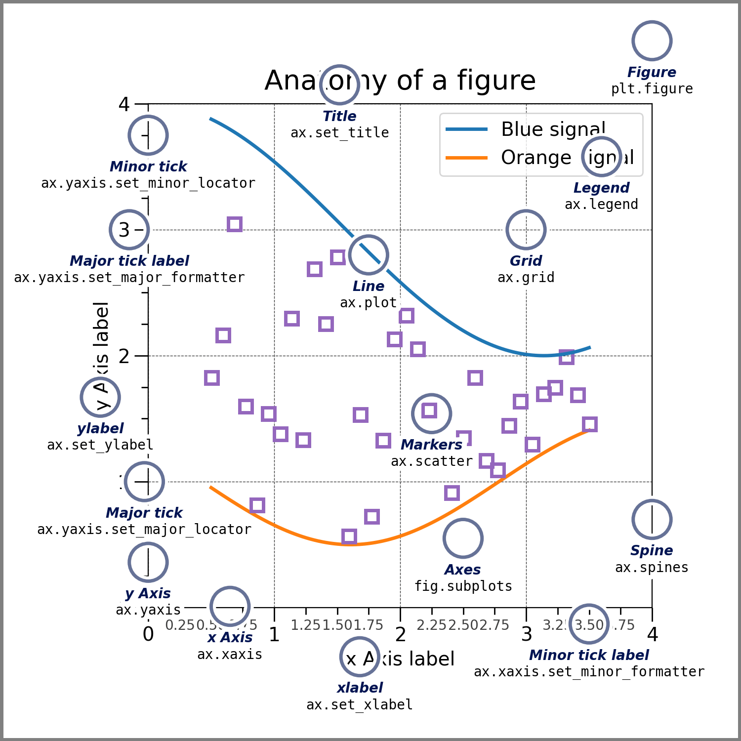
# ## Anatomy of a matplotlib figure
# > Exercise: Comment out parts of the code above and see what happens to the plot.
#
# First we load the data
# ([Source](https://matplotlib.org/stable/gallery/showcase/anatomy.html)).
# %%
np.random.seed(19680801)
X = np.linspace(0.5, 3.5, 100)
Y1 = 3 + np.cos(X)
Y2 = 1 + np.cos(1 + X / 0.75) / 2
Y3 = np.random.uniform(Y1, Y2, len(X))
data = {"X": X, "red_line": Y1, "blue_line": Y2, "circles": Y3}
data = pd.DataFrame(data)
data.head()
# %% [markdown]
# Create the figure without the annotations. Ready to customize!
# %%
from matplotlib.ticker import AutoMinorLocator, MultipleLocator
fig = plt.figure(figsize=(7.4, 7.4))
ax = fig.add_axes([0.2, 0.17, 0.68, 0.7], aspect=1)
ax.xaxis.set_major_locator(MultipleLocator(1.000))
ax.xaxis.set_minor_locator(AutoMinorLocator(4))
ax.yaxis.set_major_locator(MultipleLocator(1.000))
ax.yaxis.set_minor_locator(AutoMinorLocator(4))
ax.xaxis.set_minor_formatter("{x:.2f}")
ax.set_xlim(0, 4)
ax.set_ylim(0, 4)
ax.tick_params(which="major", width=1.0, length=10, labelsize=14)
ax.tick_params(which="minor", width=1.0, length=5, labelsize=10, labelcolor="0.25")
ax.grid(linestyle="--", linewidth=0.5, color=".25", zorder=-10)
ax.plot(X, Y1, c="C0", lw=2.5, label="Blue signal", zorder=10)
ax.plot(X, Y2, c="C1", lw=2.5, label="Orange signal")
ax.plot(
X[::3],
Y3[::3],
linewidth=0,
markersize=9,
marker="s",
markerfacecolor="none",
markeredgecolor="C4", # color 5 in color palette
markeredgewidth=2.5,
)
ax.set_title("Anatomy of a figure", fontsize=20, verticalalignment="bottom")
ax.set_xlabel("x Axis label", fontsize=14)
ax.set_ylabel("y Axis label", fontsize=14)
ax.legend(loc="upper right", fontsize=14)
# %% [markdown]
# ## Save the figure
# - file ending will decide format (and 'backend' to be used for export)
# %%
fig.savefig("anatomy_of_figure.png", dpi=300)
fig.savefig("anatomy_of_figure.pdf")
# %%
# ## Proteomics data example
# - plotting a histogram via the pandas interface
# %%
import os
import pathlib
import pandas as pd
IN_COLAB = "COLAB_GPU" in os.environ
fname = pathlib.Path("data") / "proteins" / "proteins.csv"
if IN_COLAB:
fname = (
"https://raw.githubusercontent.com/biosustain/dsp_workshop_dataviz_python"
"/refs/heads/main/data/proteins/proteins.csv"
)
df = pd.read_csv(fname, index_col=0)
df
# %%
x = df.iloc[0]
x
# %%
ax = x.hist()
# %%
fig, ax = plt.subplots()
# try to change the color
n, bins, patches = ax.hist(x, bins=30, alpha=0.7, color="C0")
# %% [markdown]
# ## Available styles
# Choose your preferred style with it's defaults
# [here](https://matplotlib.org/stable/gallery/style_sheets/style_sheets_reference.html)
#
# ```python
# plt.style.use('ggplot')
# ```
#
# 
# 
# 
# %%
with plt.style.context("ggplot"):
fig, ax = plt.subplots()
n, bins, patches = ax.hist(x, bins=30, alpha=0.7)
# %% [markdown]
# ## Exercise
# Combine two plots:
# %%
fig, axes = plt.subplots(nrows=1, ncols=2, figsize=(7.4, 4))
axes = axes.flatten() # in case of more than one dimension (safety snippet for you)
ax = axes[0]
n, bins, patches = ax.hist(x, bins=30, alpha=0.7, color="C0")
ax = axes[1]
# Add a second plot here
# %%