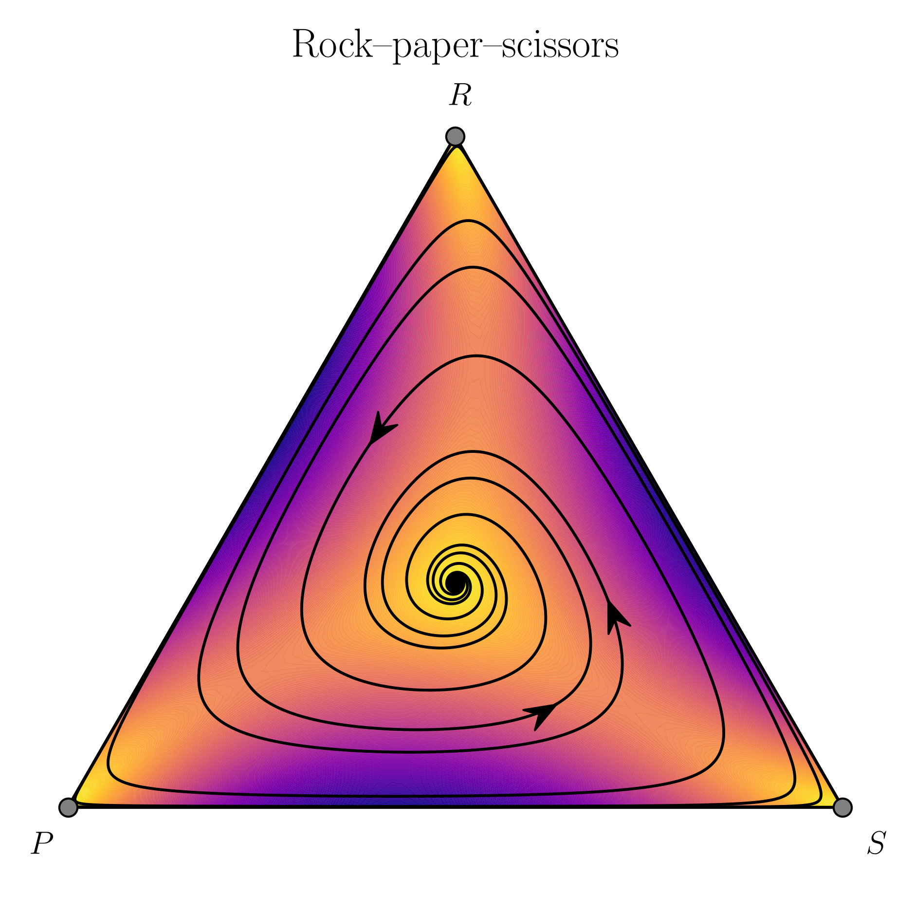
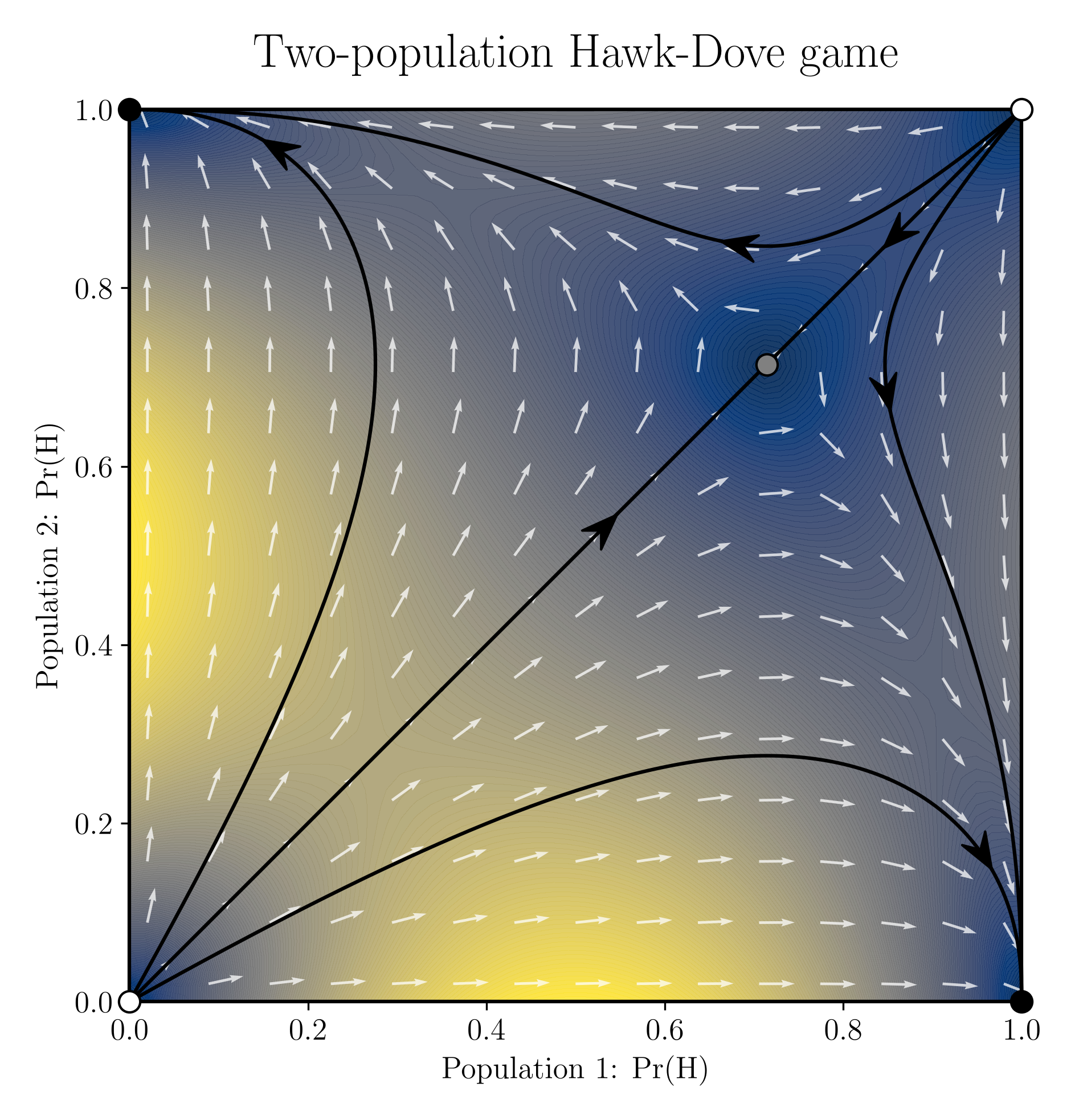
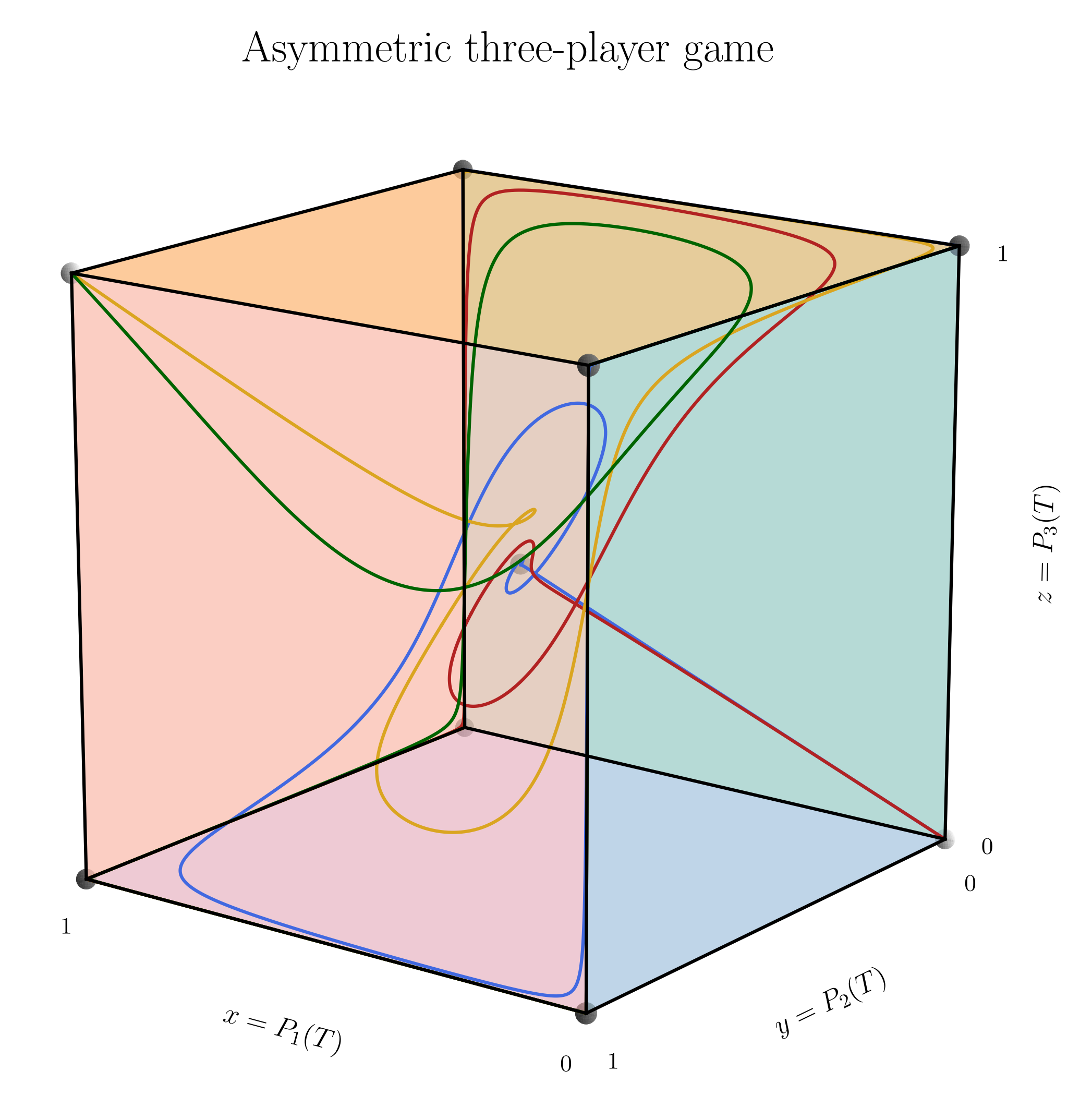
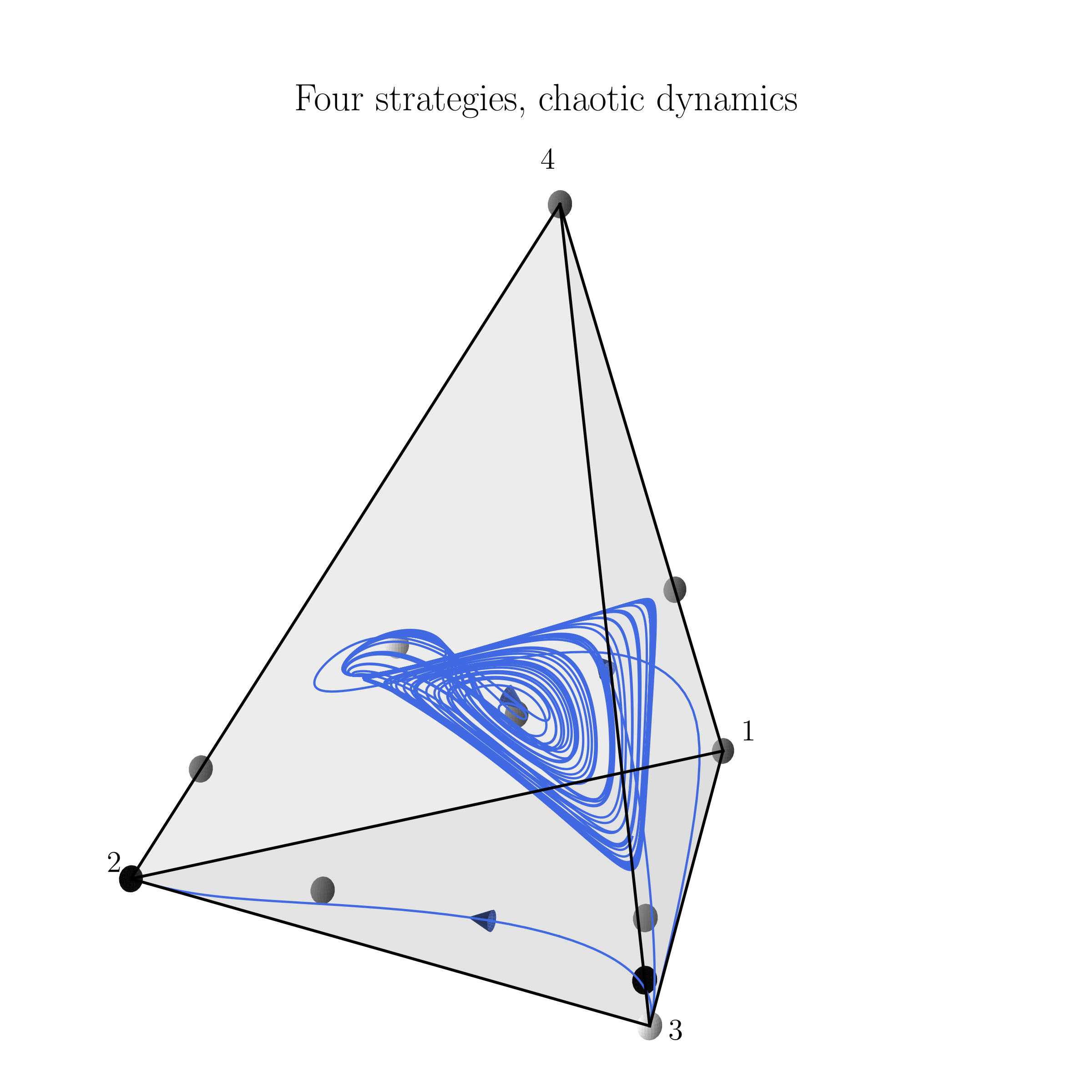
pyNamo-EGT

pyNamo-EGT is a Python package for plotting and analyzing replicator dynamics in evolutionary games. It focuses on game classes whose state spaces can be visualized directly, producing phase portraits on simplices with trajectories, speed fields, vector fields, equilibria, and stability information.

The package is designed for researchers, teachers, and students who want clear, publication-quality diagrams of theoretical phase portraits. Its high-level interface is built for Jupyter notebooks and produces informative figures with minimal code, while still exposing fine-grained controls for plotting details. Its design is inspired by Dynamo (Sandholm, Dokumacı & Franchetti), the Mathematica package for diagrams of evolutionary game dynamics, and brings that approach to the Python ecosystem.

Gallery

Start Here

There are three main ways to try pyNamo-EGT.

1. Full interactive tutorial in Binder

Use Binder if you want the closest experience to a local Jupyter notebook, including the interactive widget and rotatable 3D Matplotlib figures:

Launch the Binder tutorial

Binder runs in the browser and does not require a local installation. First launch can take a few minutes while Binder builds the environment.

Interactive 3D plots may occasionally appear blank in Binder. Try rerunning the plotting cell. If the issue persists, replace %matplotlib widget with %matplotlib inline in that plotting cell for a static preview without rotation. SVG/PDF export quality is unaffected.

2. Faster static tutorial in Google Colab

Use Colab if you want a faster browser-based preview of the tutorial:

Open the Colab tutorial

The Colab notebook supports ordinary plotting cells, but not the interactive widget or rotatable 3D Matplotlib figures.

3. Local installation from GitHub

Use a local installation if you want to use pyNamo-EGT in your own notebooks or modify the code:

git clone https://github.com/SlimaneD/pynamo.git
cd pynamo
pip install ".[notebook]"

Features

• One-population symmetric 2×2 phase lines and one-parameter bifurcation diagrams, with customizable phase-line labels and curve styles.
• Replicator dynamics for asymmetric 2-player / 2-strategy games (2Pop2S), symmetric 2-player / 3-strategy games (1Pop3S), symmetric 2-player / 4-strategy games (1Pop4S), and asymmetric 3-player / 2-strategy games (3Pop2S).
• A curated catalogue of built-in example games with descriptions, references, parameter notes, and explanations of what each example illustrates.
• Matplotlib phase portraits with trajectories, equilibria, speed fields, vector fields, and optional colored faces for 3D state spaces.
• Reproducible grid-based default trajectories, with automatic one-dimensional flow arrows on triangle and square boundaries.
• Equilibrium analysis with linear stability classification, Nash equilibria, strict Nash equilibria, and ESS checks where applicable.
• A Jupyter widget for quick exploration of built-in example games.

Installation

Requires Python 3.12+. Install from PyPI:

pip install pynamo-egt

For notebook and widget support (recommended for Jupyter users):

pip install "pynamo-egt[notebook]"

To install from source (for development or to modify the code):

git clone https://github.com/SlimaneD/pynamo.git
cd pynamo
pip install ".[dev]"
python -m pytest -q

First use

import matplotlib.pyplot as plt

import pynamo_egt as pn

fig, ax = pn.phase_portrait(pn.examples.games.good_rps)
plt.show()

pn.phase_portrait returns ordinary Matplotlib objects, so figures can be modified or saved with standard Matplotlib commands:

fig.savefig("good_rps.svg", bbox_inches="tight")
fig.savefig("good_rps.pdf", bbox_inches="tight")

Built-In Examples

Built-in games are available through pn.examples.games:

g = pn.examples.games.battle_of_the_sexes
same_game = pn.examples.games("battle_of_the_sexes")
pn.examples.games.by_class("2Pop2S")

Each catalogue game carries metadata:

g = pn.examples.games.chaotic_four_strategy_game
g.describe()

You can also use the module-level helper:

pn.examples.describe(g)

The metadata include the game description, reference, parameter values, and the main mathematical point illustrated by the example.

Game Classes

Game-class identifiers use population counts (Pop) and strategies per population (S), rather than the number of players in an interaction. A symmetric two-player interaction can be modeled in one population or in two separate populations.

pyNamo currently supports five game classes:

• 1Pop2S: symmetric 2-player / 2-strategy games in one population, represented by one 2 x 2 payoff matrix.
• 2Pop2S: 2-player / 2-strategy games, represented by one payoff matrix per player. In each matrix, rows are that player's own strategies and columns are the opponent's strategies.
• 1Pop3S: symmetric 2-player / 3-strategy games, represented by one 3 x 3 payoff matrix.
• 1Pop4S: symmetric 2-player / 4-strategy games, represented by one 4 x 4 payoff matrix.
• 3Pop2S: 3-player / 2-strategy games, represented by one 2 x 2 x 2 payoff tensor per player.

For asymmetric 2-strategy games, each coordinate in a reduced state is the probability that the corresponding player uses their first listed strategy.

For symmetric 3-strategy games, initial conditions use two coordinates and the third strategy frequency is inferred. For symmetric 4-strategy games, initial conditions use three coordinates and the fourth strategy frequency is inferred.

Defining Games

A symmetric 3-strategy game:

import numpy as np
import pynamo_egt as pn
my_game = pn.Game(
    name="My RPS Variant",
    payoffs=np.array([
        [0, -1, 2],
        [2, 0, -1],
        [-1, 2, 0],
    ], dtype=float),
    strategy_labels=["R", "P", "S"],
)

An asymmetric 2-player / 2-strategy game:

Each payoff matrix uses its recipient as the focal player. The first matrix has player 1's strategies as rows and player 2's as columns; the second has player 2's strategies as rows and player 1's as columns.

my_asymmetric_game = pn.Game(
    name="My Asymmetric Game",
    payoffs=(
        # Player 1 rows; player 2 columns.
        np.array([[3, 0], [1, 2]], dtype=float),
        # Player 2 rows; player 1 columns.
        np.array([[2, 1], [0, 3]], dtype=float),
    ),
    player_strategy_labels=[["A", "B"], ["C", "D"]],
    player_labels=["Player 1", "Player 2"],
    symmetric=False,
)

Plot Customization

Most common plotting options are parameters of pn.phase_portrait:

fig, ax = pn.phase_portrait(
    pn.examples.games.matching_pennies,
    starts=[[0.2, 0.7], [0.7, 0.5], [0.9, 0.9]],
    tmax=40,
    speed_cmap=plt.cm.cividis,
    speed_levels=20,
    show_vector_field=True,
    vector_grid=18,
    trajectory_color="black",
    trajectory_linewidth=1.2,
    trajectory_arrows=[0.001],
)

When starts is omitted, pyNamo uses deterministically spaced starts. For 1Pop3S and 2Pop2S, it also treats every invariant edge as a one-dimensional phase line and places arrows halfway between consecutive edge equilibria. Control the exact number of generated trajectories with trajectory_number; explicit starts override it. Use show_edge_flow=True to combine explicit starts with boundary flow, or show_edge_flow=False to hide boundary flow. Boundary-arrow positions are determined by edge equilibria rather than the time-based trajectory_arrows values; trajectory_arrows=[] hides all arrowheads.

Use one color per trajectory by passing a list:

fig, ax = pn.phase_portrait(
    pn.examples.games.cyclic_mismatching_pennies,
    starts=[[0.52, 0.50, 0.48], [0.70, 0.45, 0.35]],
    trajectory_color=["tab:blue", "tab:orange"],
    trajectory_arrows=[],
    tmax=1000,
)

Colored faces are available for 3D state spaces:

fig, ax = pn.phase_portrait(
    pn.examples.games.ownership_game,
    show_faces=True,
    face_alpha=0.15,
)

Vector fields are available for both 2D and 3D game classes. Sparse 3D vector fields can be useful for exploration, but trajectories are usually clearer in static publication figures.

Labels are Matplotlib text labels and can include simple LaTeX-style math notation such as "$S_1$" or "$x = P(A)$". pyNamo-EGT does not require a full LaTeX installation by default; users who want full LaTeX rendering can enable Matplotlib's text.usetex option manually.

For the full parameter documentation:

help(pn.phase_portrait)

Equilibrium Analysis

For notebooks, use pn.equilibrium_table:

import pynamo_egt as pn

pn.equilibrium_table(pn.examples.games.good_rps)

For programmatic use:

result = pn.analyze_equilibria(pn.examples.games.good_rps)
rows = result.to_rows()

For quick access to static equilibrium concepts:

pn.rest_points_nash(game=pn.examples.games.good_rps)
pn.rest_points_strict_nash(game=pn.examples.games.good_rps)
pn.rest_points_ess(game=pn.examples.games.good_rps)

These helpers filter the replicator rest points detected by pyNamo; they do not claim to enumerate additional or non-isolated Nash-equilibrium families. rest_points_ess returns ESS only for symmetric games.

Stability Caveats

Stability is classified from the linearization restricted to admissible directions in the state space. This is important at boundaries because outward perturbations are not valid evolutionary deviations.

Some equilibria are non-hyperbolic or belong to degenerate equilibrium sets. In these cases pyNamo emits warnings rather than forcing a classification. For higher-dimensional games, non-isolated equilibrium manifolds are not plotted automatically; isolated equilibria are still shown when they can be identified.

The category unstable means that linearization proves the equilibrium is not stable, but does not always distinguish source from saddle. In plots, unstable equilibria are drawn with the source color for visual compatibility.

Interactive Widget

In a notebook, use:

%matplotlib widget

import pynamo_egt as pn
pn.interactive.launch_replicator_widget()

The widget lets users choose a game class and example, adjust trajectories, toggle speed/vector fields, and inspect payoff data and equilibrium analysis.

If 3D rotation does not work, make sure the notebook kernel has ipympl installed and that %matplotlib widget has been evaluated.

Related software and acknowledgements

pyNamo's design is directly inspired by Dynamo (cited in full below), the Mathematica package for evolutionary game dynamics diagrams by Sandholm, Dokumaci, and Franchetti. Users who prefer Mathematica or need features not yet in pyNamo should consult Dynamo first.

W. H. Sandholm, E. Dokumaci, and F. Franchetti (2012). Dynamo: Diagrams for Evolutionary Game Dynamics. http://www.ssc.wisc.edu/~whs/dynamo.

Several Python packages cover related but distinct ground:

• EGTtools (Fernández, 2023) — finite-population stochastic evolutionary dynamics (Moran process, pairwise comparison), fixation probabilities, and stationary distributions. Complements pyNamo for stochastic simulations; the two share a common payoff-matrix convention and can be used together.
• Nashpy — Nash equilibrium computation for 2-player games via support enumeration and Lemke–Howson. Complements pyNamo's equilibrium visualization with rigorous exhaustive enumeration.
• egtplot — simplex plots of replicator dynamics for 3-strategy games in Python; the closest predecessor to pyNamo's simplex functionality.

Repository Structure

• pynamo_egt/game.py: core Game class and game-class inference.
• pynamo_egt/examples.py: curated catalogue of predefined games.
• pynamo_egt/dynamics.py: replicator vector fields and rest-point computation.
• pynamo_egt/analysis.py: equilibrium and stability analysis.
• pynamo_egt/drawer.py: plotting helpers and phase_portrait.
• pynamo_egt/interactive.py: Jupyter widget front-end.
• tutorial.ipynb: notebook tutorial.
• tests/: pytest test suite.

One-population phase lines and bifurcation diagrams

coordination = pn.Game("Coordination", [[1, 0], [0, 1]], strategy_labels=["A", "B"])
fig, ax = pn.phase_portrait(coordination, figsize=(8, 2.2))

fig, ax = pn.bifurcation_diagram(
    lambda s: [[s, 0], [1, 2]],
    parameter_range=(-1, 4),
    parameter_values=[1],
    phase_line_values=[0, 2, 3],
    phase_line_labels=["I", "II", "II"],
    stable_linestyle="-", unstable_linestyle="--",
)

For phase lines, x is the first strategy's frequency. trajectory_arrows=None centers one head between equilibria; explicit values are frequencies, and [] hides heads. Marker styling follows the existing API. continuum_color styles an entire stationary interval. Non-hyperbolic isolated points are classified from one-sided flow without special markers or warnings.

Bifurcation diagrams sample a payoff-matrix function; they do not guarantee exhaustive bifurcation detection. See the two introductory tutorial sections and help(pn.bifurcation_diagram) for styling and parameter controls.

Possible future directions

pyNamo focuses on analytical models whose state spaces can be visualized. Natural extensions include:

• More evolutionary dynamics and learning rules. Refactor dynamics.py around updating-rule objects, allowing each population or player to have its own rule. Candidate additions include logit dynamics, best-response dynamics, and differential equations for reinforcement learning and stochastic fictitious play.
• Nonlinear frequency-dependent fitness. Accept user-defined fitness functions $f_i(x)$ in addition to payoff matrices.
• Equilibrium manifolds. Detect continua of rest points, analyze their stability, and plot them automatically when the result can be established reliably. Report inconclusive cases explicitly.