


A multi-resolution landscape connectivity algorithm for calculating Habitat Connectivity (Connected-Habitat), PARC Connectedness and the Bioclimatic Ecosystem Resilience Index (BERI).
This algorithm operates on the overview layers of raster files which are now generated on-the-fly.
The package is published on PyPI as eco-connectivity (NOTE: pip install connectivity installs an unrelated package):
pip install eco-connectivityThe import name is still connectivity:
from connectivity import connectedness, beriTo build the latest development version from the GitHub repository, install Rust first, then run:
git clone https://github.com/csiro/connectivity.git
cd connectivity
pip install .Resolve the bundled example paths once so they can be reused throughout the analysis:
from connectivity import beri, connectedness, example_data_path, resolution_info

condition_file = example_data_path("site_condition")
pa_file = example_data_path("pa_proportion")
current_file = example_data_path("transgrids/1990")
future_files = [
    example_data_path("transgrids/IPS50_45"),
    example_data_path("transgrids/GFD50_85"),
]
To bound the spatial extent of the connectivity calculation, the algorithm limits how far it searches across neighboring cells in the condition raster. The approximate one-sided search reach is computed as:
max_reach = outer_window * max(levels) * resolution. For example, with a 1 km resolution raster, a max-level of 32, and an outer_window of 11, the resulting search reach is:
distance = outer_window × max_level × resolution
         = 11 × 32 × 1 km
         = 352 km
Use resolution_info() to preview how candidate levels will change raster
dimensions and approximate search reach before running the analysis:
resolution_info(condition_file, outer_window=9)File: .../connectivity/data/site_condition.tif
Base raster: 588 x 516 cells (303.41K total)
Base resolution: 0.008333 degrees
CRS: EPSG:4326
Bands: 1
Data type(s): float32
Nodata: -9999.0
Outer window: 9
Small-dimension warning threshold: < 16 cells
Distance note: approximate km values use centre latitude -41.550
Candidate internally generated levels:
Level Width Height Cells % base Resolution Reach Reach km Note
1 588 516 303.41K 100.000% 0.008333 degrees 0.075 degrees 8.349 km
2 294 258 75.85K 25.000% 0.01667 degrees 0.15 degrees 16.7 km
4 147 129 18.96K 6.250% 0.03333 degrees 0.3 degrees 33.4 km
8 74 65 4.81K 1.585% 0.06667 degrees 0.6 degrees 66.79 km
16 37 33 1.22K 0.402% 0.1333 degrees 1.2 degrees 133.6 km
32 19 17 323 0.106% 0.2667 degrees 2.4 degrees 267.2 km
64 10 9 90 0.030% 0.5333 degrees 4.8 degrees 534.3 km small grid; review
128 5 5 25 0.008% 1.067 degrees 9.6 degrees 1.07K km small grid; review
256 3 3 9 0.003% 2.133 degrees 19.2 degrees 2.14K km small grid; review
512 2 2 4 0.001% 4.267 degrees 38.4 degrees 4.27K km small grid; review
The default window_mode="circular" uses source-centered circular annuli with
fractional area/count support at annulus boundaries. The
window_mode="square" option uses the same source-centered fractional
construction with square annuli. These modes change indicator values, so
compare outputs only between runs that use the same window mode.
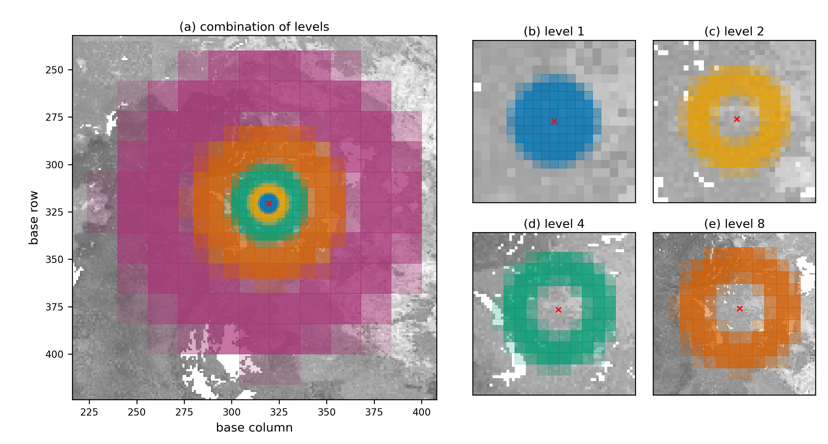
Each coloured neighbourhood represents a different raster aggregation level. Fine levels capture nearby cells at higher resolution, while coarser levels extend the search over larger distances. Their contributions are combined into a single graph, in which the least-cost path from the focal cell is calculated for each aggregated cell. See Valavi et al. (2026) for the full method.
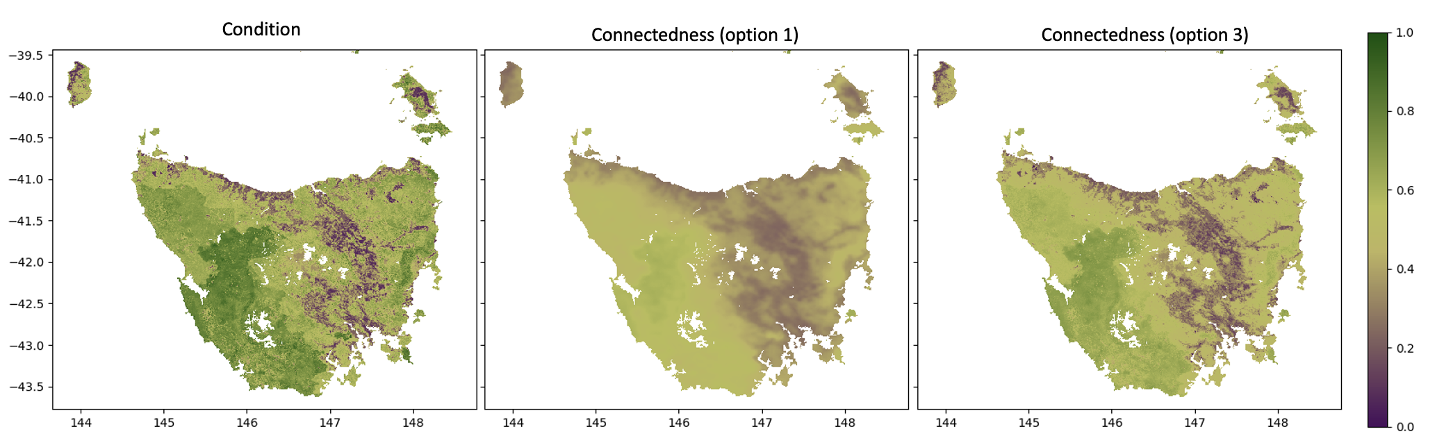
To compute connected-habitat (or plain connectedness), you only need a habitat condition raster. Use option argument to generate the connected-habitat from connectedness and input condition with:
connectednessconnectedness * conditionsqrt(connectedness * condition)— geometric mean (default)
connd = connectedness(
    condition_file = condition_file,
    lambdas = [2, 20, 200],
    max_cost = 2.0,
    window_size = 5,
    outer_window = 11,
    window_mode = "circular",
    levels = [2, 4, 8, 16, 32],
    option = 3,
    filename = "./results/connected_habitat.tif"
)
By default the habitat condition raster does double duty: it weights how costly each cell is to
move through and supplies the habitat value used in the indicator. Pass an optional
resistance_file to decouple these two roles. The resistance raster (values in [0, 1],
higher = harder to cross, scaled with resistance_scale) then drives only the least-cost path
traversal, while condition still supplies the habitat value:
connd = connectedness(
    condition_file = condition_file,
    resistance_file = resistance_file,   # optional; decoupled movement-cost surface
    resistance_scale = None,             # divide resistance into [0, 1] if needed
    max_cost = 2.0,
    window_mode = "circular",
    levels = [2, 4, 8, 16, 32],
)
The edge weight becomes w = (1.0 - max_cost) * (1 - resistance) + max_cost, so resistance = 0
is free (w = 1) and resistance = 1 is the most costly (w = max_cost). When resistance_file
is omitted, condition is used for traversal as before, and the output is unchanged. Cells valid in
condition but missing a resistance value fall back to condition for traversal and raise a warning,
so the analysis domain is never changed silently. The same resistance_file / resistance_scale
arguments are available on beri().
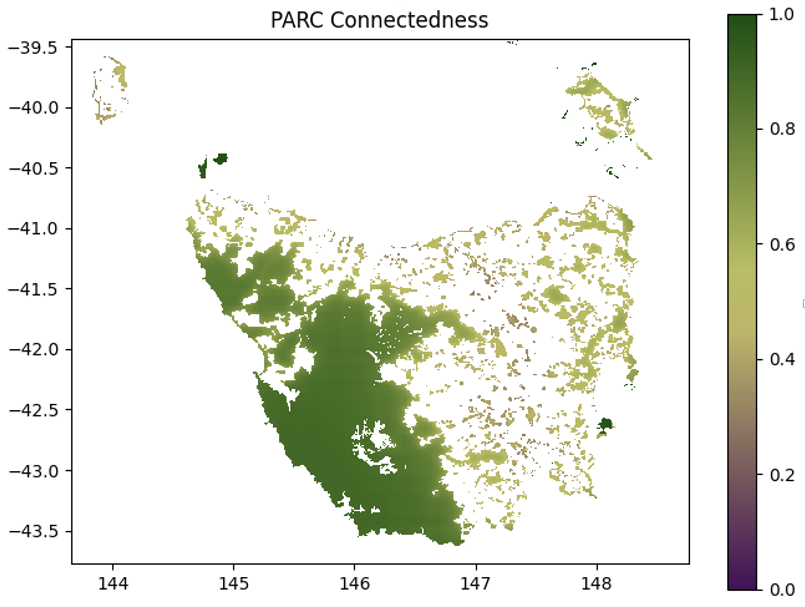
To compute PARC-connectedness, provide both:
- a habitat condition raster, and
- a protected-areas proportion raster.
When pa_file (proportion of protected-areas in each cell) is supplied, the function automatically returns PARC-connectedness instead of standard connectedness.
parcc = connectedness(
    condition_file = condition_file,
    pa_file = pa_file,
    lambdas = [2, 20, 200],
    max_cost = 2.0,
    window_size = 5,
    outer_window = 11,
    window_mode = "circular",
    levels = [2, 4, 8, 16, 32],
    filename = "./results/parc_connectedness.tif"
)
Use pixel_coverage() when you need the proportion of each raster pixel covered
by polygon geometry. The calculation is backed by a performant Rust
implementation:
from connectivity import pixel_coverage

coverage = pixel_coverage(
    "./data/polygons.gpkg",
    condition_file,
)To compute BERI, you must provide:
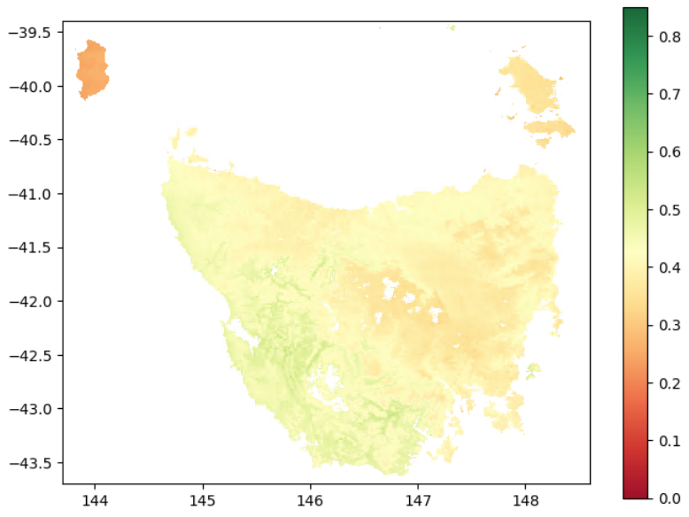
- a condition raster
- current GDM transgrids
- one or more future transgrids scenarios (as a list)
beris = beri(
    condition_file = condition_file,
    current_file = current_file,
    future_files = future_files,
    lambdas = [2, 20, 200],
    max_cost = 2.0,
    window_size = 5,
    outer_window = 11,
    window_mode = "circular",
    levels = [2, 4, 8, 16, 32],
    filename = "./results/berri.tif"
)
To run the model using tiles, create a rectangular tile polygon as a GeoDataFrame
and pass it to the polygon_mask argument. This limits data loading to only the
portion required for the tile, i.e. the output core plus the internally buffered
neighborhood.
Use make_tile() to generate non-overlapping output-core tiles whose internal
boundaries align with the coarsest aggregation level. This is preferred over
creating overlap-expanded tile polygons externally. Be sure to set
closed_border = False (the default) so that neighborhood information is
included around each tile core.
from connectivity import connectedness, make_tile

levels = [2, 4, 8, 16, 32]

tile_id = 0
tile_poly = make_tile(
    raster_file = condition_file,
    nrows = 4,
    ncols = 4,
    tile_id = tile_id,
    align_to = max(levels),
)

connd = connectedness(
    condition_file = condition_file,
    polygon_mask = tile_poly,
    closed_border = False,
    margin_px = 32,
    lambdas = [2, 20, 200],
    max_cost = 2.0,
    window_size = 5,
    outer_window = 11,
    window_mode = "circular",
    levels = levels,
    option = 1,
    filename = f"./results/connected_habitat_tile_{tile_id}.tif"
)
For large, uneven workloads, use balanced tiles:
tile_poly = make_tile(
    raster_file = condition_file,
    nrows = 4,
    ncols = 4,
    tile_id = tile_id,
    align_to = max(levels),
    balanced = True,
    io_weight = 0.1,
)
Balanced tiling uses a deterministic raster-mask cost estimate while preserving
the same align_to boundary alignment. It is useful for global rasters where
some tiles contain mostly ocean or nodata and others contain many valid land
pixels. Use balanced = False (the default) when equal aligned tiles are enough.
When balanced = False, io_weight is ignored.
To cite connectivity library in publications and reports, please use:
Valavi, R., Mokany, K., Ware, C., Vickers, M., Giljohann, K. M., & Ferrier, S. (2026). A scalable multi-resolution framework for connectivity-based biodiversity indicators. EcoEvoRxiv. https://doi.org/10.32942/X2S68V