
Recent advancements in computer vision underscore the need for large, labeled datasets to develop robust and efficient deep learning-based vision models. However, creating such extensive datasets through manual annotation is both cost-prohibitive and impractical due to the highly imbalanced nature of real-world datasets, where negative samples, which are of minimal interest, predominate. In this work, we introduce the Iterative Reverse Image Search (IRIS) algorithm, an iterative approach designed to alleviate the data annotation burden significantly. We propose a search algorithm that combines Nearest Neighbor search and a modified Diversity Sampler on the embeddings of pre-trained self-supervised models to discover samples similar to a given query sample. These components collaboratively guide the annotator to label only those samples identified as likely positive, thereby reducing the labeling of negative samples and accelerating the discovery of new samples while minimizing human effort. Although the idea can be easily extended to any domain, we strictly confine ourselves to computer vision here.
-
Unlabelled Dataset:
$\mathbb{D}_{\text{images}}$ The complete set of all unlabelled images available to the algorithm. -
Seed Samples: A small set of initial samples selected from
$\mathbb{D}_{\text{images}}$ , which are used as a reference. The algorithm attempts to find samples similar to these. -
Positive Samples: Samples from
$\mathbb{D}_{\text{images}}$ that are labelled (by the annotator) to belong to the same class as the seed samples. Any set of positive samples is denoted by a+in the superscript eg$A^+$ -
Negative Samples: Samples from
$\mathbb{D}_{\text{images}}$ that are labelled (by the annotator) to belong to a different class than the seed samples. Any set of negative sample is denoted by a-in the superscript eg$A^-$ -
Feature Extractor:
The feature extractor is the pre-trained backbone that converts images into feature vectors. It is denoted by$f_{\text{enc}}$ . -
$f_c$ (MLP Head):
A single-layer MLP head that maps the latent space to$\mathbb{R}$ , typically used to assign confidence scores or make predictions based on the feature representations. -
Latent Dataset (
$\mathcal{D}$ ):
The full dataset is represented in the latent space:
-
Labelled Set (
$\mathcal{L}$ ):
The set of all labelled samples (both positive and negative) grows over successive annotation rounds. -
Discovered Positives (
$\Lambda$ ):
The subset of$\mathcal{D}^+$ identified and labelled as positive by the annotator. -
Discovery Rate (Recall Rate) (
$d_r$ ): The discovery rate is the proportion of positive samples discovered:
-
Labelling Efficiency (Precision) (
$L_e$ ): The ratio of discovered positive samples to the total labelled samples:
- Composite Metric: A geometric mean of the above two metrics (precision and recall):
Before beginning our discussion on the search algorithm and its associated technicalities, it is essential first to convert our images into embeddings. These embeddings serve several crucial purposes:
-
Dimensionality Reduction
Images are inherently high-dimensional objects with a large number of degrees of freedom. Converting them into compact, dense representations allows us to address the curse of dimensionality while significantly reducing computational overhead. The resulting embeddings form a compressed yet information-rich representation of the original image space, making the subsequent search both efficient and accurate. -
Metric Definition in Embedding Space
Each embedding corresponds to a point in$\mathbb{R}^n$ , and the relative orientation and magnitude of these vectors capture intrinsic similarities between the original samples. This establishes a well-defined metric space, where distances between points correlate with semantic similarity in the original image domain. Thus, embeddings not only encode semantic information but also provide a geometrical interpretation of similarity, which is essential for constructing an effective search algorithm. -
Formation of Clusters
The embeddings tend to form clusters, where samples with similar features are mapped close to each other. This clustering property implies that once a single point within a cluster is identified, one can infer the approximate nature of other points in that region. The concept of a metric and direction in the embedding space, therefore, allows for efficient exploration and retrieval of similar samples.
To convert our image to embeddings, we primarily use VICReg. The working of VICReg is discussed in the following section.
VICReg: Variance-Invariance-Covariance Regularization for Self-Supervised Learning work by training on the surrogate task of generating embedding spaces that are invariant to specific augmentation spaces. This is achieved by using a Siamese-like setup, where two views of the same event are used, but both have been augmented to different degrees. The Euclidean distance in the embedding space between these two views is then minimised using gradient descent.
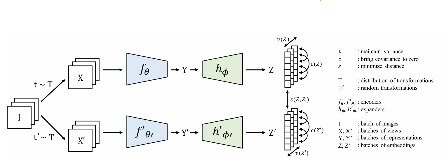
Along with the MSE loss that acts across the two projection vectors Z, to ensure stability against collapse and the non-triviality of the embedding space, we have the Covariance and Variance regularisation terms. The covariance component prevents the embedding dimensions from capturing the same information. In contrast, the variance component prevents all embedding vectors in a batch from collapsing to a single point in the representation space.
Given that the image dataset has now been converted into embeddings, we next discuss the nature of clustering within the embedding space. For a given seed sample
To elaborate further, consider an example scenario using the ImageNet dataset, denoted as
where each class
Following the discussion so far, one might quickly realize that using a K-nearest neighbor search on the embedding space might be the solution to this optimization problem. Although the former is partially true, one cannot discover all the samples belonging to a single class solely by using a nearest neighbor type search algorithm. The argument can be further understood by examining the clusters more closely within the embedding space.
-
Sparse Clusters:
Embedding algorithms such as VICReg are known for their ability to cluster semantically similar samples closely while simultaneously pushing dissimilar ones farther apart. In the ideal limit of perfect optimization, one would expect all samples belonging to the same class to collapse into a compact cluster, with inter-cluster centers maximally separated in the latent space. The compactness, or “tightness,” of a cluster can thus be defined by the relative distances between any two samples within the same class.Conversely, under suboptimal training conditions, both intra-cluster compactness and inter-cluster separation deteriorate, eventually approaching complete randomness as the model becomes less ideal. Practically, most embedding algorithms operate in an intermediate regime, where clusters are not perfectly compact and their centers are not well-separated. This results in partial overlap and contamination between clusters due to the presence of negative samples (belonging to different classes) within the neighborhood of positive ones.
Such overlap directly impacts labeling efficiency, especially in nearest–neighbor–based search algorithms, where the number of samples within a given search radius increases exponentially with the radius.
-
Multiple Disconnected Clusters:
The samples belonging to a desired class may often be distributed across multiple, potentially disjoint, clusters within the embedding space. Continuing with the ImageNet example consisting of classes${ C_0, C_1, \dots, C_n} $ , it is possible that the search objective is to identify all samples corresponding to a composite class such that$C^* = C_a \cup C_b \cup C_c$ . A representative case would be the discovery of all images of mammals within the ImageNet dataset. In such scenarios, the nearest-neighbour search remains constrained to a local region of the embedding space and, consequently, fails to retrieve samples lying in spatially disconnected clusters. This inherent locality limits the overall effectiveness of the search process in capturing the complete semantic diversity of the target class. -
Boundary Queries:
Seed samples originating near the boundary of a cluster, within a latent space of dimension
$N$ , inherently require a large search radius due to the scaling of hypervolume with radius as$r^N$ . As a result, moving away from the cluster centroid leads to an exponential decline in search efficiency. -
Out-of-Cluster Queries:
If a query sample lies outside any cluster, the nearest neighbour search mechanism completely fails. Furthermore, as the query moves farther from the cluster centre, the computational effort required to locate similar samples increases exponentially.
To maximize the efficiency of the search, we need two components within the search algorithm. We need a nearest neighbour-like search to explore the proximity of a given positive sample to find more positive samples from the surroundings, which we call the Spread Sampler (SpreadS). We need a stochastic sampler or a diversity-type search that tries to sample new points that are far away from this cluster. The Stochastic or Random Like Sampler, which we call Cluster Search (ClusterS), attempts to find new Clusters that the Spread Sampler can explore in later iterations.
We present the following modified variant of the nearest neighbor search algorithm, which samples positive samples from the surroundings.
Input:
Output:
$\mathcal{D}' \gets \mathcal{D} \setminus (\Lambda \cup S)$ - Set
$\mathcal{M}[i,j] = \text{MSE}(\mathcal{D}'[i], S[j])$ -
For each
$i$ :
$\mathcal{R}[i] = \min \left( \bigcup_j \mathcal{M}[i,j] \right)$ $\mathcal{R}^* = \text{arg sort}_{\text{ascending}}(\mathcal{R})$ -
$\delta \gets$ first$a$ samples of$\mathcal{R}^*$ -
Return
$\mathcal{D}'[\delta]$
The above implementation of the nearest neighbour sampling works slightly differently from a vanilla KNN algorithm. In the said algorithm, we have a hyperparameter
The task of ClusterS, or the diversity sampler, is to identify new data points belonging to previously undiscovered clusters associated with the same class as the seed samples. To estimate the likelihood of a point belonging to the seed class, a Multi-Layer Perceptron (MLP) head is trained on the already identified positive samples. The objective of ClusterS is to discover samples that exhibit a high probability of being positive—belonging to the same class—while simultaneously residing sufficiently far away on the embedding space from the already discovered cluster centers. The Cluster Search method, therefore, attempts to optimise the following criteria to achieve the most effective and diverse sampling of positive points.
-
$M_1$ : The likelihood of being positive. This component of the optimisation criterion ensures that the diversity sampler returns only those samples that have a high probability of being a positive sample, and not random samples.
-
$M_2$ : The distance between each drawn sample. This component ensures that, in a single sampling step, the diversity sampler returns samples from as many different sources as possible.
-
$M_3$ : The distance between each drawn sample with the positive labelled samples$\Lambda$ . This component ensures that the diversity sampler indeed returns samples from clusters far away from those already discovered.
In the above equations,
The total cost that needs to be maximized is
When
In this work, we explore how to solve this optimisation problem to define an optimal search algorithm.
In this section, we develop the GridS algorithm, which can serve as a suitable candidate for the diversity sampler or ClusterS. Later, we also discuss another parallel algorithm called RandS, which can be used as a diversity sampler too. Here, we limit our discussion to GridS.
The Cluster Search algorithm must maximize the three components of the cost function that we described in previous sections, coupled with the Spread search, to work optimally. Formulating analytic solutions to the above optimization is challenging. We try to find an approximate algorithmic solution to the above problem.
We begin by dividing the entire embedding space into grids by segmenting the first few principal components of the embedding space. To address the second component of the equation, we strictly select only one sample from each grid. Now we have the first and the last component of the problem remaining. We scrutinize it and realise that the two are inversely linked to one another, given that the confidence of the MLP head is bound to decrease as the distance of the selected point from the already labelled samples on which the MLP head was trained increases. This makes it possible for us to rewrite the joint optimisation criterion, excluding the second component, as:
By fine-tuning and empirically finding the value of
Input:
Output:
-
Step 1: Dimensionality Reduction Using PCA
$\mathcal{D}{red} \gets \text{PCA}(\mathcal{D}, m)$ Let $\mathcal{D}{red} = {(x_{1i}, x_{2i},..., x_{mi}) \mid i = 1, 2, \dots, n}$
i.e.$n$ points with coordinates$(x_1, x_2,..., x_m)$ -
Step 2: Partition the Dataset along Each Dimension
For each$j \in {1, 2, \dots, m}$ :
a. $\mathcal{R} \gets \mathcal{D}{red}$
b. $\mathcal{R} \gets \text{argsort}{i=1}^n \mathcal{R}[i][j]$
c. For each$k \in {1, 2, \dots, N}$ :
i.$D_{kj} \gets \mathcal{R}\Big[\dfrac{(k-1)n}{N} : \dfrac{kn}{N}\Big]$ -
Step 3: Define Blocks
$L \gets [\ ]$
For each$k \in {1, 2, \dots, N^m}$ :
a. $B_k = \Big{\bigcap\limits_{l=1}^n \bigcap\limits_{j=1}^m \mathcal{D}{k[l]j} \ \big| \ k \text{ is an m-string on } {1, 2, \dots, N}\Big}$
b. $f_c(v) \gets \zeta f{MLP}(v) + (1 - \zeta)\big(\min\limits_{l \in \Lambda}{|l - v|}\big)$, where$\Lambda$ is the set of discovered positive samples.
c.$f_c(B_k) = \max{f_c(v) \mid v \in B_k}$
d.$L.\text{append}(B_k, f_c(B_k))$ -
$L = \text{sort}(L)$ w.r.t.$f_c(B)$ for$B \in L$ -
Output:
$L[N^m - s : -1]$ #$s$ samples
We return to our discussion of the complete three-component cost function. This time, we aim to develop a simpler algorithm by further relaxing the boundaries of our assumption. We return to the second component of our cost and claim that if we randomly draw samples from the dataset, then we can automatically ensure that all the samples are well spread apart, given a large number of samples are selected. This is equivalent to setting the value of
Input:
Output:
-
For each
$\mathcal{D}[i]$ in$\mathcal{D}$ :
a.$H_i \gets \text{Head}(\mathcal{D}[i])$ -
$T \gets \text{Mean}(H) + \alpha \times \text{Stdev}(H)$ -
$S \gets {\mathcal{D}[i] \mid H_i > T}$ -
$S \gets \text{Select } b \text{ random samples from } S$
-
Return
$S$
Now, given that we have developed all the associated components of our search algorithm, we define the complete algorithm as follows:
Input:
Output:
$\delta^0 \gets \Lambda$ -
For
$i = 1$ to epochs:
a.$K \gets \text{SpreadS}(\delta^0, a)$
b.$\delta \gets \text{ClusterS}(\mathcal{D}, b)$
c.$\gamma \gets K \cup \delta$
d.$\text{Oracle}(\gamma) \to (\gamma^+, \gamma^-)$
e.$\Lambda \gets \Lambda \cup \gamma^+$
f. Train MLP head on$(\Lambda \cup \gamma^-)$
g.$i \gets i + 1$ -
For each
$\mathcal{D}[i]$ in$\mathcal{D}$ :
a.$H_i \gets \text{Head}(\mathcal{D}[i])$ $T \gets \text{Mean}(H) + \alpha \times \text{Std}(H)$ $z \gets {\mathcal{D}[i] \mid H_i > T}$ $\text{Oracle}(z) \to (z^+, z^-)$ $\Lambda^* \gets \Lambda \cup z^+$ -
Return
$\Lambda^*$
In the above algorithm, we begin with a few seed samples that we denote by
To assess the strengths and limitations of our algorithm, we evaluate it on the ImageNet dataset. We first compute embeddings for all images using a pretrained VICReg encoder. For each evaluation setting, we uniformly sample 50 classes at random and attempt to recover all samples belonging to those classes, given a fixed budget of initial query examples. We sweep the query budget over {1, 2, 5, 10, 50}. For each budget, we run five independent random seeds and repeat the entire procedure five times to address statistical noise.
We have discussed in the previous sections how the nearest neighbor algorithm alone is not sufficient for discovering all the samples associated with our search query. Here, we present our findings after evaluating just the nearest neighbour search component over two different radii of searches.
| No. of seeds | LE (a=50) | D (a=50) | GM (a=50) | LE (a=200) | D (a=200) | GM (a=200) |
|---|---|---|---|---|---|---|
| 1 | 0.15 | 0.0323 | 0.0696 | 0.1233 | 0.0369 | 0.06745 |
| 2 | 0.15 | 0.0331 | 0.0704 | 0.1461 | 0.0573 | 0.09149 |
| 5 | 0.24 | 0.0761 | 0.1351 | 0.1707 | 0.0723 | 0.11109 |
| 10 | 0.26 | 0.0661 | 0.1310 | 0.1786 | 0.1046 | 0.13668 |
| 50 | 0.41 | 0.1173 | 0.2193 | 0.2866 | 0.1176 | 0.18358 |
Note: LE = labelling efficiency; D = discovery rate; GM = geometric mean.
Spread search, being a nearest-neighbour exploration, has a relatively low discovery rate but a high labelling efficiency. We evaluate our algorithm for two different search (a = 50) and (a = 200). Given that there exist two different evaluation components to maximize, we try to combine them into a single composite metric by calculating the Geometric Mean between the two. We will compare this composite score across all different algorithms.
To supplement our SpreadS algorithm, we add a random search algorithm to it. We begin by just adding a simple random sampler to the search algorithm. If we refer back to our original cost function:
By simply having a random sampler, we are effectively eliminating the first term, or setting the value of
| No. of seeds | LE | D | GM |
|---|---|---|---|
| 1 | 0.03408 | 0.85384 | 0.17059 |
| 2 | 0.03520 | 0.88153 | 0.17617 |
| 5 | 0.03381 | 0.88423 | 0.17290 |
| 10 | 0.03395 | 0.89153 | 0.17398 |
| 50 | 0.02829 | 0.93538 | 0.16268 |
Compared to a simple nearest neighbor search, we can already see that the composite score has increased for most cases, except for the case with 50 different seeds. This can be explained by the fact that the nearest neighbour search improves as it has more initial cluster centers to begin with, given that it gets access to almost all the clusters, making the need for a diversity sampler redundant.
Next, we attempt to evaluate the complete RandS algorithm, which was discussed in detail in the previous section.
| No. of seeds | LE | D | GM |
|---|---|---|---|
| 1 | 0.1204 | 0.8861 | 0.3266 |
| 2 | 0.1205 | 0.8819 | 0.3260 |
| 5 | 0.1159 | 0.8659 | 0.3169 |
| 10 | 0.1141 | 0.8713 | 0.3153 |
| 50 | 0.1058 | 0.8969 | 0.3082 |
We can clearly see that this combination of algorithms outperforms all the previous ones. Even for a vast number of initial seed examples, the algorithm outperforms the simple nearest neighbour search. The reason behind this can be explained by the fact that with a large number of initial high-quality seed/query samples, the MLP head learns the correct parameters relatively quickly, making the confidence prediction more accurate.
Finally, we present our findings on the complete algorithm using the GridS algorithm, which promises to maximise all three components of the cost function explicitly. The complete cost function for the optimisation problem is mainly dependent on two independent hyperparameters, which are:
-
N: The number of grids that we break the embedding space into. N is inversely proportional to the
$\beta$ parameter in the original equation. -
$\zeta$ : The parameters$\alpha$ and$\gamma$ are dependent on each other, and the overall cost can be simplified into a two-component form, which is controlled by the parameter$\zeta$ .
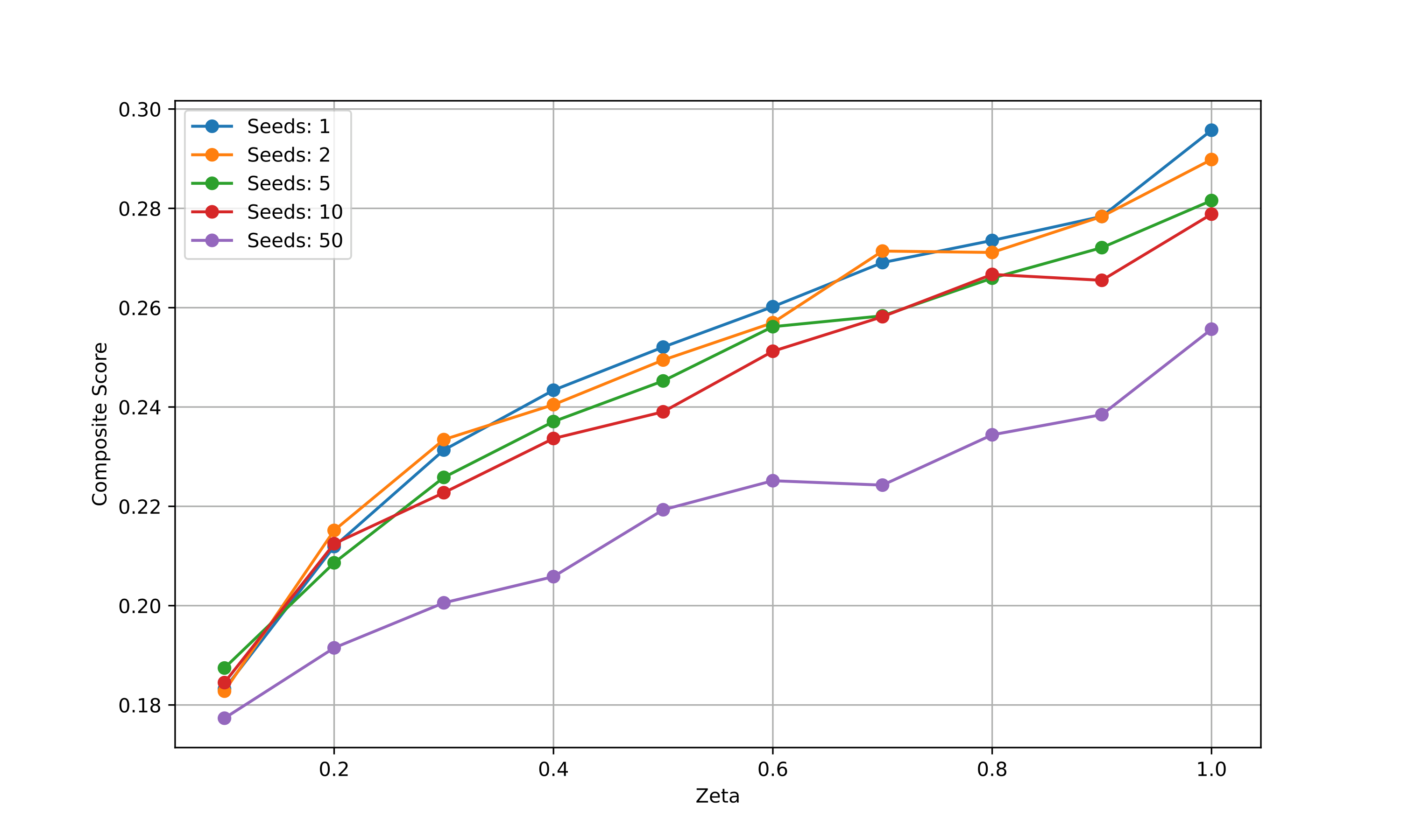
Determining the above two parameters accurately will ensure that our algorithm works perfectly. Given the excessive cost of running the experiment for multiple variants of
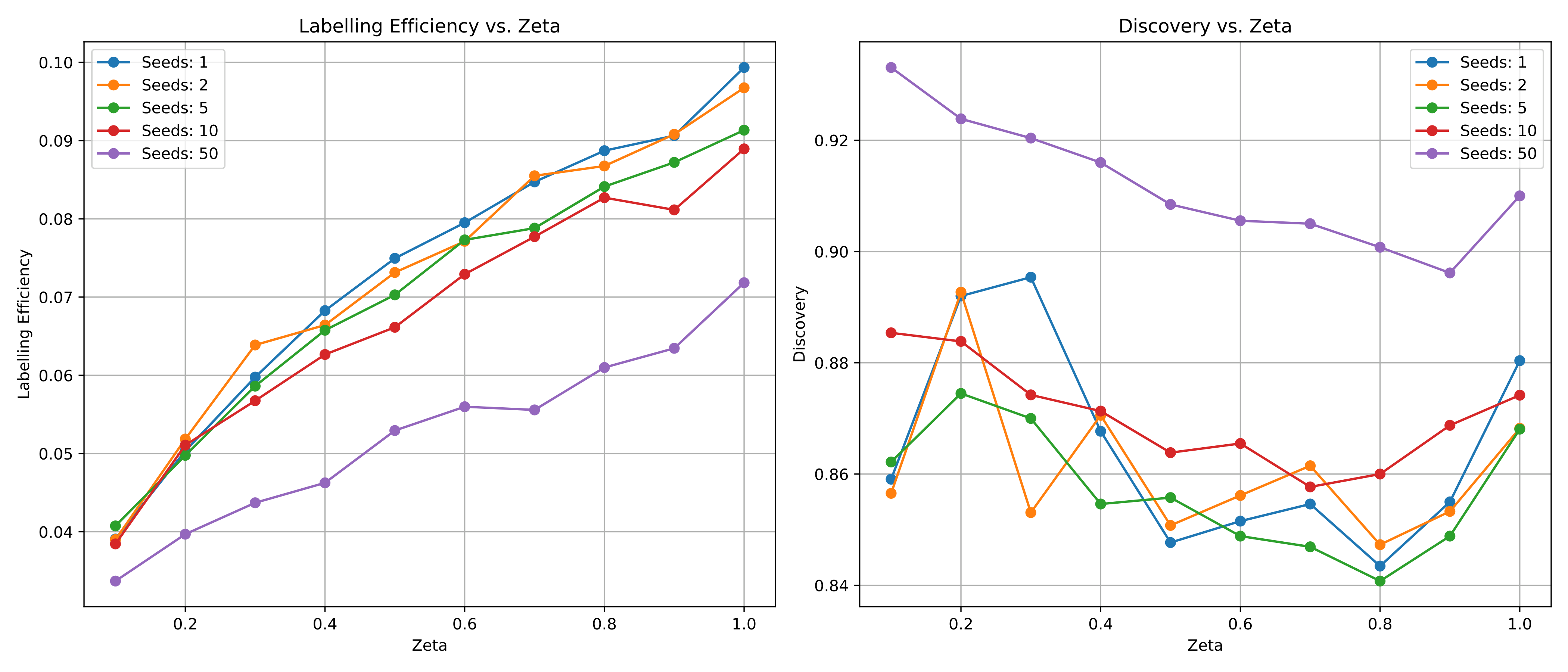
The above plot shows that the labelling efficiency monotonically increases as the value of
Now, we compare the performance of all the different algorithmic combinations that we have discussed so far.
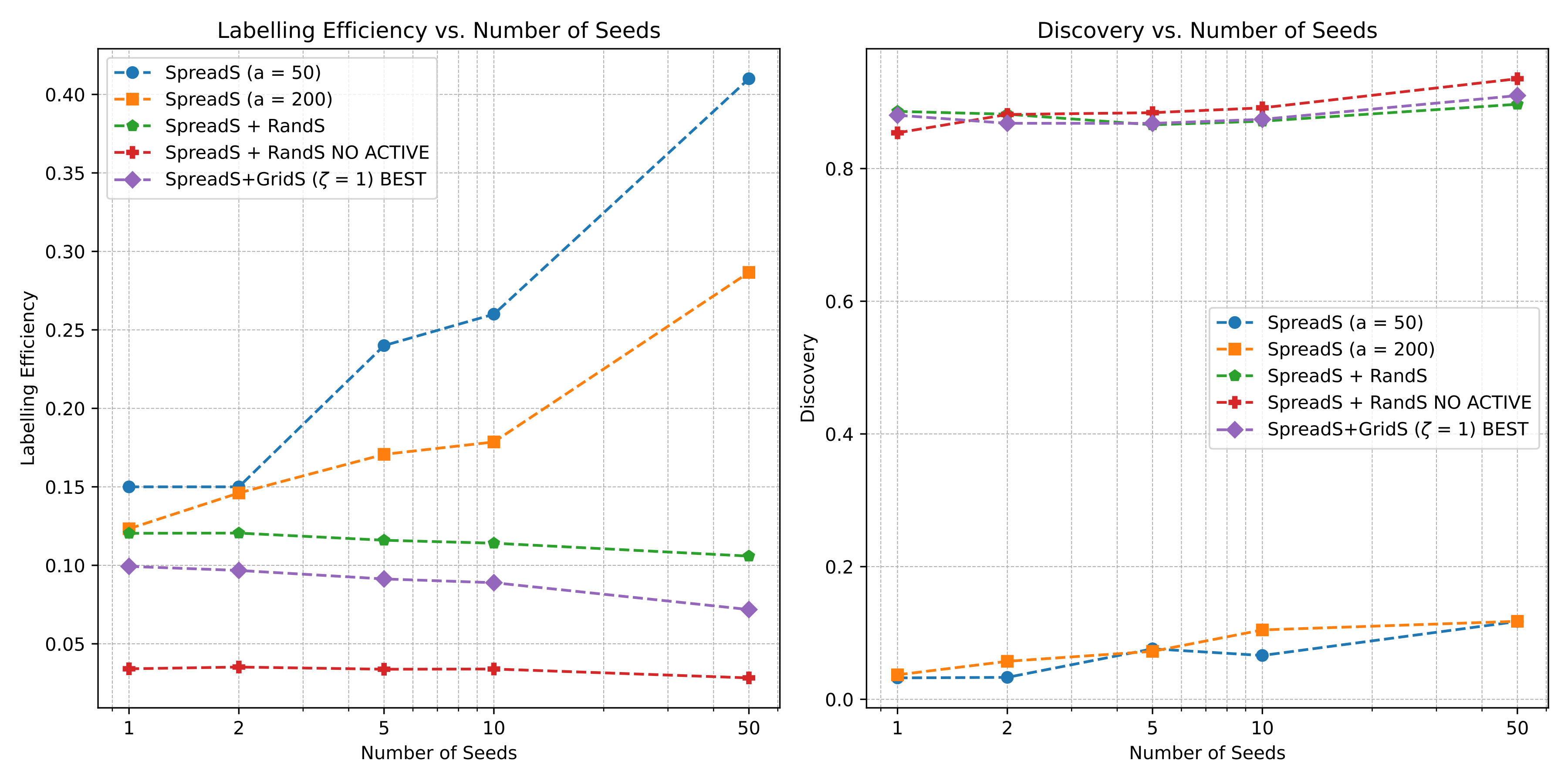
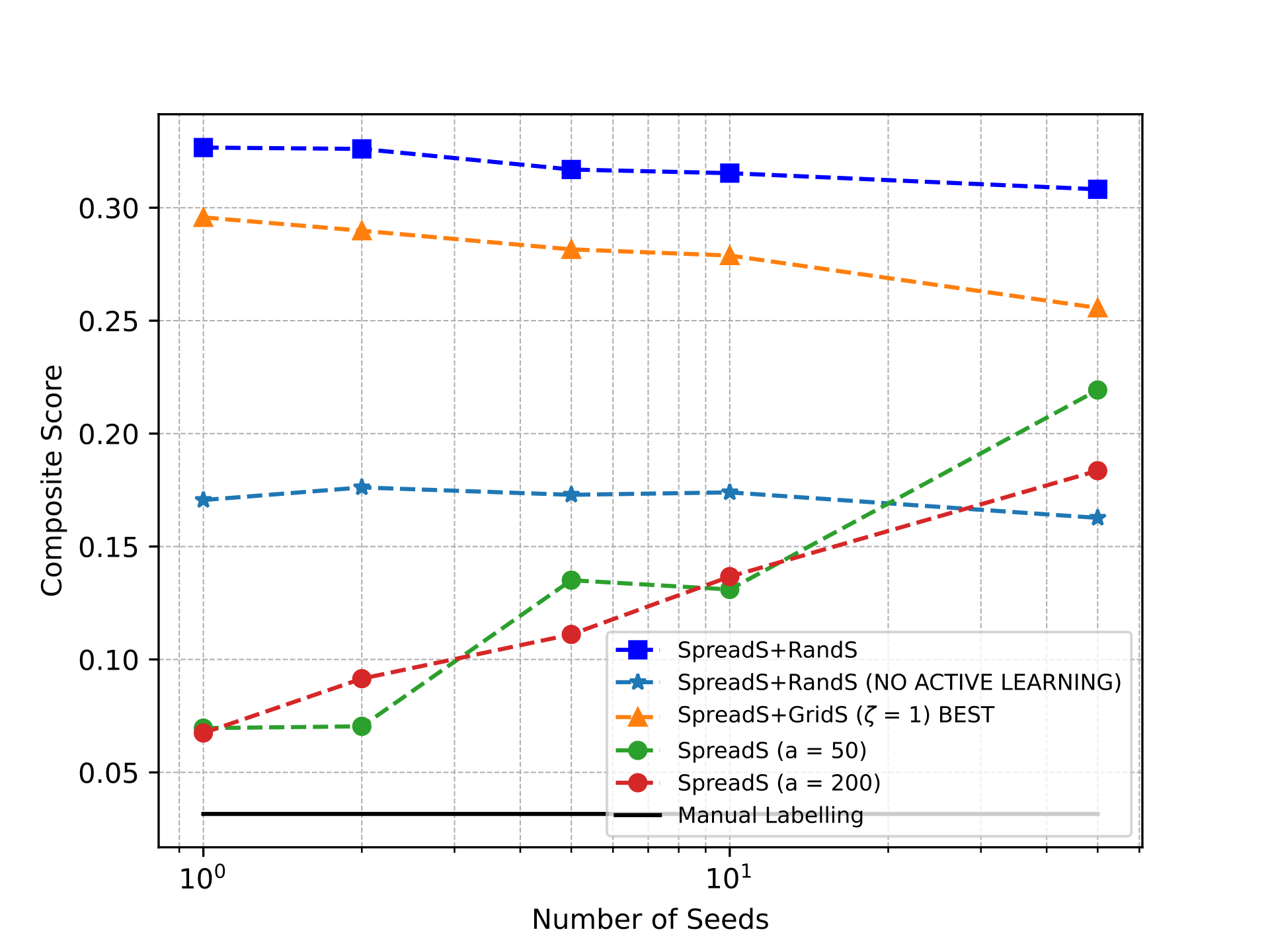
As shown in the above plots, the RandS component, when used as a diversity sampler, performs slightly better than grid-like sampling. This is evident from the fact that the GridS had the optimal value of the
In this work, we developed the IRIS framework to alleviate the task of manual labelling by combining nearest neighbour type search with a suitable diversity sampler. We discussed two different types of diversity samplers, both of which demonstrate superior performance compared to the existing nearest neighbor type or manual labeling baselines. IRIS can be used to expedite the curation of new datasets and citizen science-type projects where manual labeling is essential. The values of the hyperparameters that have been extensively discussed throughout this work can be tuned using existing labels in a large, mostly unlabelled dataset. In our future work, we aim to explore how this approach plays out by using ImageNet 1k to tune the parameters and utilizing the same dataset to label the entirety of ImageNet 22k. Datasets, such as iNaturalist, can be used to determine the parameters of the search algorithm, which can later be used to curate datasets (or identify) of endangered/rare species.